1. Java Primitive Types are bad for Learners

    This year I am teaching Java to first semester students. My own Java introduction has happened seven years ago. As I am quite interested in principles of programming languages I try to convey my enthusiasm for the topic and base my didactic methods around that. It's cool what we do. Let's talk about it.

    I see the problems in a lecture for first semester students as they have yet to learn any theoretical basis for object oriented programming, that would be useful. In my oppinion one should start with the theoretical basis, like class hierarchies and the object model. But students only learn about partial orders (like a class hierarchy) later in the first year. So ideally (in my mind at least), a computer science education is without a computer for the first semester.

    And because there is no theoretical basis, the approach taken by the professor is quite practical, and just barely supported by theory (wherever possible, but that's not much). This means that after the first lesson, students already know what a Hello World program looks like and they can fiddle with it. Even though they do not know what a class is, a static method, even methods or functions at all.

    This leads to further problems down the road. We have an online platform where students have to solve programming assignments during seminars and as homework. But since they don't know about classes and class methods (or types or return statements for that matter), we can't have them implement classes, methods, or interfaces as homework and have to have them write output into the main method. That's a bad start, when you consider programming best practices.

    Ideally one would like to start implementing small methods without function calls that implement some interface and then go on in creating more complex programs later on. But the problem is, that there is no way to run the java code without a main method. And even if you provide one, then the students can not really practice.

    This shows how necessary a REPL or interactive interpreter is.

    But Java has a few more problems that are quite bad for learners and can lead to confusion and misunderstanding.

    Some Types are Keywords

    For legacy reasons, Java has two kinds of types. There are primitive types that correspond in some manner to machine types, and the reference types that form the class hierarchy. Examples of primitive types would be int or float or void (Unit - only allowed as method return type). In general it's also the case that operators work on primite types but do not for reference types (exceptions apply). Those primitive types are builtin insofar that their type names are keywords as well.

    As a homework for the second week I gave the following task: write a program that reads a number between 0 and 100 from the standard input (they don't know about standard input yet, and I'd prefer passing arguments as command line parameters but was overruled) and write a 10 character progress bar, visualizing the progress that correspond to the input number. This is my solution I worked from:

    import java.util.Scanner;
    
    class Progress {
      public static void main(String[] args) {
        Scanner input = new Scanner(System.in);
    
        int progress = input.nextInt() / 10;
        int rest = 10 - progress;
    
        while (progress > 0) {
          System.out.print("|");
          progress = progress - 1;
        }
        while (rest > 0) {
          System.out.print("-");
          rest = rest - 1;
        }
      }
    }
    

    Since this is quite complicated for beginners, I've given them the basic structure and removed all keywords, replacing them with % and replacing all variable names with #. Resulting in this:

    import java.util.Scanner;
    
    % Progress {
      % % % main(String[] #) {
        Scanner # = % Scanner(System.in);
    
        % # = #.nextInt() / 10;
        % # = 10 - #;
    
        % (# > 0) {
          System.out.print("|");
          # = # - 1;
        }
        % (# > 0) {
          System.out.print("-");
          # = # - 1;
        }
      }
    }
    

    And as you can see, not entirely all type information is removed by replacing the keywords with #. If all types were reference types, we'd have a program that looked more like this:

    % Progress {
      % % Unit main(String[] #) {
        Scanner # = % Scanner(System.in);
    
        Integer # = #.nextInt() / 10;
        Integer # = 10 - #;
    
        % (# > 0) {
          System.out.print("|");
          # = # - 1;
        }
        % (# > 0) {
          System.out.print("-");
          # = # - 1;
        }
      }
    }
    

    Now doesn't this look quite a bit better? Some types are introduced as keywords but all user-created ones are not (and by user-created, I also mean the standard library). This is an inconsistency that is quite hard to explain away, even more so if you have yet to introduce the students to the vocabulary to explain this.

    There are even more problems quite soon. Once conditionals are introduced, we have the next problem. The language construct if () then {} else {} only works with the bool type as conditionals. So primitive types are necessary to use the language constructs for conditional execution (while as well, but the numeric comparison follows somewhat naturally).

    I do not know whether we will get this far, but for type parameters (for for polymorphic types, like containers) the primitive types don't work either.

    All in all, I'd say Java would need to do away with primitive types and consistently use reference types. But for this to work properly with the operators, one would probably also need to add operator overloading. Once you're there, you could think long and hard about whether you'd really need the new keyword for instance construction.

    And of course, one would want to introducing a proper Unit type. But since in Java all types are inhabited by the value null (who the hell had that idea?), this would be useless. So I will allow keeping the void keyword.
  2. Finding Trade and Exchange Possibilities with Prolog

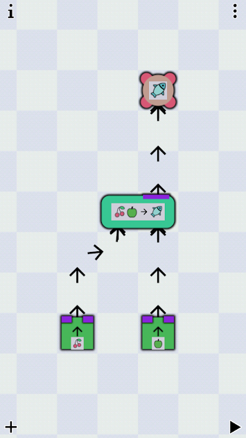
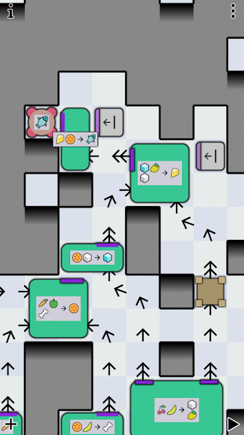
    A friend recently had an interesting problem for me: There's a game for mobile phones where you have to exchange or transmute wares into each other, in order to create some strange supply chain.

    Simple example exchanging Apple and Cherry for Fish

    Example of an earlier level.

    A very complex later example

    A very complex later example.


    The game is bleentoro, image copyright by them.

    In this example (an earlier level) the goal is to create fish. We can transmute or exchange (I will only write about exchange from now on) an apple and a pair of cherries for a fish. Apple and cherry we have, or are created from thin air, in the context of the game. As you can see in the other example, this can get very complex.

    The question is, given some input we have, in what order do we have to use the stations for exchange to create some output. How do we best model this problem?

    Modeling the Problem

    From a previous article we already know that we can encode numbers in Prolog terms using Peano numbers. Using these we can match terms that represent at least or exactly some number. Exactly 3 would be s(s(s(z))) while at least 3 would be s(s(s(X))) with the variable X representing the rest of the term for some \(n\) so that \(3 + x = n\).

    Let's start with a small example: we have an aunt that gives us apples. We have bob who is willing to exchange an apple for two berries. And we have a cousin who will bake a cake if we give them two apples and five berries.

    Let's formalize our rules in some way:

    a: / -> 1A
    b: A -> 2B
    c: 2A, 5B -> 1C
    

    We model this as some kind of inventory(A, B, C) with some slots for Peano encoded numbers. Meaning that inventory(s(z), z, s(C)) means an inventory of exactly one apple, zero berries, and at least one cake. Lucky us.

    Let's define our possible exchanges as Prolog facts with exchange(Kind, Pre, Post) meaning we use the exchange method Kind and we get from inventory state Pre to inventory state Post. If we lose an item, we have it in Pre but don't in Post. If we gain one, it's the other way around. Of course, the rest of our inventory should stay the same.

    exchange(a, inventory(A, B, C), inventory(s(A), B, C)).
    exchange(b, inventory(s(A),B,C), inventory(A, s(s(B)), C)).
    exchange(c, inventory(s(s(A)), s(s(s(s(s(B))))), C), inventory(A, B, s(C))).
    

    As we can see, we can encode basically any numeric condition that uses only "just exactly" and "at least", as well as addition and subtraction and "setting" fields to specific values. If we have to give at least three apples, but all of them, to get a cake, the rule would be exchange(c, inventory(s(s(s(_))), B, C), inventory(z, B, s(C)))..

    Programming the Solver

    We want to create a predicate trades(Start, Goal, Path) where we give a Start inventory and a Goal inventory and want to get a Path of exchanges. The most obvious approach is the following:

    trades(Goal, Goal, []).
    trades(Start, Goal, [H|T]) :- exchange(H, Start, Temp), trades(Temp, Goal, T).
    

    So we're done when our Goal is reached. And if not, we have to try some exchange. We try it and we quickly learn that...

    ?- trades(inventory(z, z, z), inventory(_, _, s(z)), Path).
    ERROR: Out of local stack
    

    ... it doesn't work.

    The problem is, that calling the exchange predicate in the recursive call always tries the first rule first and since that basically always works, we get into an infinite loop. Let's reorder the rules and put the generating rule first.

    ?- trades(inventory(z, z, z), inventory(_, _, s(z)), Path).
    ERROR: Out of local stack
    

    It still doesn't work. Let's look at the trace.

    [trace]  ?- trades(inventory(z, z, z), inventory(_, _, s(z)), Path).
     Call: (8) trades(inventory(z, z, z), inventory(_700, _702, s(z)), _712) ? creep
     Call: (9) exchange(_960, inventory(z, z, z), _984) ? creep
     Exit: (9) exchange(a, inventory(z, z, z), inventory(s(z), z, z)) ? creep
     Call: (9) trades(inventory(s(z), z, z), inventory(_700, _702, s(z)), _962) ? creep
     Call: (10) exchange(_978, inventory(s(z), z, z), _1002) ? creep
     Exit: (10) exchange(b, inventory(s(z), z, z), inventory(z, s(s(z)), z)) ? creep
     Call: (10) trades(inventory(z, s(s(z)), z), inventory(_700, _702, s(z)), _980) ? creep
     Call: (11) exchange(_1000, inventory(z, s(s(z)), z), _1024) ? creep
     Exit: (11) exchange(a, inventory(z, s(s(z)), z), inventory(s(z), s(s(z)), z)) ? creep
     Call: (11) trades(inventory(s(z), s(s(z)), z), inventory(_700, _702, s(z)), _1002) ? creep
     Call: (12) exchange(_1018, inventory(s(z), s(s(z)), z), _1042) ? creep
     Exit: (12) exchange(b, inventory(s(z), s(s(z)), z), inventory(z, s(s(s(s(z)))), z)) ? creep
     Call: (12) trades(inventory(z, s(s(s(s(z)))), z), inventory(_700, _702, s(z)), _1020) ? creep
     Call: (13) exchange(_1040, inventory(z, s(s(s(s(z)))), z), _1064) ? creep
     Exit: (13) exchange(a, inventory(z, s(s(s(s(z)))), z), inventory(s(z), s(s(s(s(z)))), z)) ? creep
     Call: (13) trades(inventory(s(z), s(s(s(s(z)))), z), inventory(_700, _702, s(z)), _1042) ? creep
     Call: (14) exchange(_1058, inventory(s(z), s(s(s(s(z)))), z), _1082) ? creep
     Exit: (14) exchange(b, inventory(s(z), s(s(s(s(z)))), z), inventory(z, s(s(s(s(s(s(z)))))), z)) ? creep
     Call: (14) trades(inventory(z, s(s(s(s(s(s(z)))))), z), inventory(_700, _702, s(z)), _1060) ? creep
     Call: (15) exchange(_1080, inventory(z, s(s(s(s(s(s(z)))))), z), _1104) ? creep
     Exit: (15) exchange(a, inventory(z, s(s(s(s(s(s(z)))))), z), inventory(s(z), s(s(s(s(s(s(z)))))), z)) ? creep
     Call: (15) trades(inventory(s(z), s(s(s(s(s(s(z)))))), z), inventory(_700, _702, s(z)), _1082) ? creep
     Call: (16) exchange(_1098, inventory(s(z), s(s(s(s(s(s(z)))))), z), _1122) ? creep
    

    We're still running into an infinite loop since we're just getting apples and trading them for berries.

    There's a trick if our solution is a list. If the length(List, Length) predicate is called with both predicates free (length(L, _) for example), we get lists of increasing length as solutions. So if we can bind our solution to lists of increasing length, we won't get infinite loops of apple-berry-exchanges without ever trying short solutions.

    So our query now looks like this:

    ?- length(Path,_), trades(inventory(z, z, z), inventory(_, _, s(z)), Path).
    Path = [a, b, a, b, a, b, a, a, c] ;
    Path = [a, b, a, b, a, a, b, a, c] ;
    Path = [a, b, a, b, a, a, a, b, c] ;
    Path = [a, b, a, a, b, b, a, a, c] ;
    Path = [a, b, a, a, b, a, b, a, c] ;
    Path = [a, b, a, a, b, a, a, b, c] ;
    Path = [a, b, a, a, a, b, b, a, c] ;
    Path = [a, b, a, a, a, b, a, b, c] ;
    Path = [a, b, a, a, a, a, b, b, c] ...
    

    As it turns out, there are a few ways to do it, but nothing shorter than 9 trades. We can even look, whether we have anything left over after we got our cake:

    ?- length(Path,_), trades(inventory(z, z, z), inventory(A, B, s(z)), Path).
    Path = [a, b, a, b, a, b, a, a, c],
    A = z,
    B = s(z) .
    

    Yeah. As it turns out, we have a berry to spare.

    Conclusion

    This is how you do it. And of course, you could simulate a shop with that, as one inventory slot could be the number of coins. If the inventory gets too large, you can split it into item types so you don't have to copy every unchanged item from the pre-condition to the post-condition. Then you can copy a term that might represent any number of items.

    But beware: this algorithm (with Prolog's evaluation scheme) has not so good complexity. For a solution of length \(n\) and \(m\) rules it has a run time of \(O(m^n)\). We create every possible solution list permutation but break early, if no rules are applicable.

    Depending on our instantiation of Start and Goal, this algorithm doesn't terminate (if the system isn't terminating, the algorithm isn't either). Our system doesn't terminate as we can always apply a again and again. We're creating increasingly longer partial solutions which might turn out to be no solution at all. If there is no solution, you won't know. The algorithm just tries longer and longer lists trying to find a solution.

    If you have any other conditions on your solution (some exchanges might be limited or necessary) you can put most of them after the trades call. Some conditions, like membership, can be put before.

    Let's say we have a terminating system by taking away the a rule. If our Start is fully instantiated, then our algorithm terminates. Let's try another query and find out, with how many apples we need to start to get a cake:

    ?- trades(inventory(A, z, z), inventory(_, _, s(z)), Path).
    ERROR: Out of local stack
    

    Through the unification rules, it is possible that a rule creates terms on the left side of the rule. In this case, the algorithm tries to give us increasing amounts of berries to match that with the starting condition (only rule b is applied in reverse, always leaving us with one cake, which doesn't match the starting condition). There we need the length predicate.

    ?- length(Path,_), trades(inventory(A, z, z), inventory(_, _, s(z)), Path).
    Path = [b, b, b, c],
    A = s(s(s(s(s(_2334))))) .
    

    We need at least five apples for a cake. But we knew that.


    To recap:

    • We saw again how useful it is, to encode the natural numbers in a term structure.
    • A solver is easily written but the algorithm isn't fast.
    • The rules can be applied in both directions because of Prolog's evaluation scheme. This leaves queries that would intuitively work divergent.
    • By using the length predicate we can simulate breadth-first evaluation, while the default evaluation scheme is depth-first.

    I think, there's a different approach using linear programming. I might try that in the future.


  3. Haskell Countdown Solver

    I love watching 8 Out Of 10 Cats Does Countdown. It's a british panel show where a few comedians solve word puzzles and mathematics puzzles. It's based on the game show Countdown that's been running since 1982.

    And I also like the host Jimmy Carr very much.

    The Puzzles

    The show consists of three different puzzles:

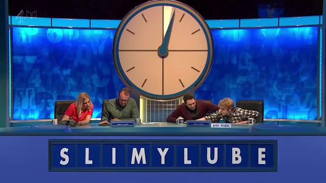
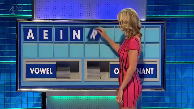
    In the Letters round a team (or single contestant) picks 9 consonants and vowels from their respective piles. After the team chooses from one of both piles, the letter is revealed and put up on the board. They then choose again until 9 letters are on the board. After all letters are on the board, the teams have 30 seconds to form a word out of as many of the letters as possible. The team with the longest word scores that many points.

    Letters round

    Letters Round

    In the Conundrum a list of letters that already spell out a funny group of words is given by the host and the contestants try to find a 9 letter anagram. The first team to buzzer in the correct answer gains 10 points. This is the final round of the game.

    Conundrum

    Conundrum

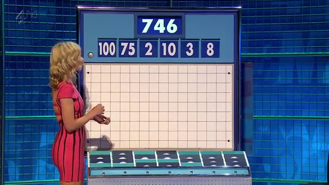
    In the Numbers round a team (or single contestant) picks 6 numbers from two piles. A random number is picked and the contestants have to create a mathematical formula out of the picked numbers that equal the target number. The specific rules follow.

    Numbers round

    Numbers Round

    Numbers Round

    According to Wikipedia there are 6 columns of 4 numbers (4 rows). One column contains the numbers 25, 50, 75, and 100 and the other 5 columns contain the numbers 1 to 10 twice each. That's not exactly the same as on the show, as there appear to be 7 columns of 4 numbers but not every stack has all 4 number cards.

    Contestants choose a total of 6 numbers from the "small" and "large" columns. The usual pick would be 2 to 3 "large" numbers and the rest small ones.

    Then a random number between 100 und 999 is generated. The contestants try to create a mathematical formula that has the random number as the result. In the formulare only the following operations are allowed:

    • Addition
    • Multiplication
    • Subtraction (that does not result in a negative number)
    • Division (that results in an integer)

    The contestants do not have to use all the numbers to get the target number.

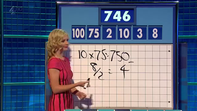
    Finished Numbers round

    Finished Numbers Round

    Since I am really not good at this, I wrote a solver for the numbers game in Haskell.

    Solver

    How do we go about this problem? First of all, we have to decide on a data structure. Let's start with a traditional term structure where a Term is a binary operation and two terms, or an integer value. An Operation is the function mapping two integers to a third, and a string to pretty-print the operation. The mapping is not total and might fail.

    data Term = Op Operation Term Term | Val Integer
    data Operation = Operation {fun :: (Integer -> Integer -> Maybe Integer), name :: String}
    
    instance Show Term where
      show (Val x) = show x
      show (Op op l r) = "(" ++ (show l) ++ (name op) ++ show r ++ ")"
    

    Now we have to define our operations and what they should do. Since we're using Maybe, and it's a monad, we can use monadic notation where it suits us:

    operations = [  Operation (\x y -> return (x + y)) "+"
                 ,  Operation (\x y -> return (x * y)) "*"
                 ,  Operation (\x y -> guard (x > y) >> return (x - y)) "-"
                 ,  Operation (\x y -> guard (x `mod` y == 0) >> return (x `div` y)) "/"
                 ]
    eval :: Term -> Maybe Integer
    eval (Val v) = Just v
    eval (Op o l r) = do l' <- eval l
                         r' <- eval r
                         (fun o) l' r'
    

    As we can see, the preconditions to the subtraction and division are encoded using the guard function. If the function returns true, the whole operation returns Nothing, otherwise it returns Just the value.

    Since Haskell uses lazy evaluation, we can define a list of all possible terms given a list of integers and filter for the ones that evaluate to the correct number.

    As we create a Term we have to be careful to not use any of the numbers again. So we will split our numbers in two sets. One that can be used in the left Term of an Operation and the rest can be used in the right Term. We will create all terms using our definition. A Term is either the Value of one of the numbers for that subterm, or an operation with some numbers reserved for the left term and some numbers reserved for the right term.

    terms :: [Integer] -> [Term]
    terms nums =  do  n <- nums -- choose a number
                      [Val n] -- one solution
                  ++
                  do  op <- operations -- choose an operation
                      (l, r) <- subset_split nums -- choose a split
                      guard $ l /= []
                      guard $ r /= []
                      ls <- (terms l) -- choose a term for the left side
                      guard (eval ls /= Nothing)
                      rs <- (terms r) -- choose a term for the right side
                      guard (eval rs /= Nothing)
                      [Op op ls rs] -- one solution
    

    For performance reasons we already evaluate the generated subterms in order to check whether the operations are valid. There are a lot of terms that can not be evaluated and we want to throw them out as early as possible (or not even generate them).

    We haven't defined subset_split yet. The idea is, to just split the list of numbers in two groups in every possible way:

    subsets :: [Integer] -> [[Integer]]
    subsets []  = [[]]
    subsets (x:xs) = subsets xs ++ map (x:) (subsets xs)
    
    subset_split nums = do l <- subsets nums
                           return (l, nums \\ l)
    

    Now all that remains is to generate all terms given a set of numbers, evaluate them, filter out the ones that don't have the correct value, and return the first one:

    solve :: [Integer] -> Integer -> Maybe Term
    solve nums target = let possible_solutions = map (\x -> (x, eval x)) (terms nums)
                            solutions = filter (\x -> (snd x) == (Just target)) possible_solutions
                        in listToMaybe $ map fst solutions
    

    And in our main we only read the list of numbers and the target as arguments and print the solution:

    main = do args <- getArgs
              let nums = (read (args !! 0))::[Integer]
                  target = (read (args !! 1))::Integer
              print $ solve nums target
    

    And there we go:

    $ ./countdown "[100, 75, 2, 10, 3, 8]" 746
    Just (8+(3+((75*(100-2))/10)))
    

    Our solution is \(8+3+{{75*(100-2)} \over 10}\) while the solution from the show was \(10*75 - {8 \over 2}\).

    As you can see, we do not always get the easiest solution but we usually have a solution quite fast. This one took about a tenth of a second. The 30 seconds given to the contestant are usually quite enough. To make sure we had the "nicest" solution, we probably would need to generate all terms and sort them by size. The smallest one should be the nicest one.


  4. Prolog Programs, Order of Evaluation, and Functional Equivalents

    While teaching Prolog this semester I had a few thoughts about Prolog programs and their equivalent programs in a functional programming language like Haskell.


    The Peano Naturals

    The Peano numbers are a unary number system for positive natural numbers where the zero is represented by a Z (or 0, or any atom - it doesn't matter) and every successor of a natural number N is the function S applied to N. We would therefore represent the natural number 3 with the term S(S(S(Z))). To look at it differently: in the Peano axioms, the naturals are defined as the set that contains zero and a closure over the successor function. In haskell we would define the type of the naturals like this:

    data N = Z | S N
    

    In Prolog we don't need a type definition for the naturals, as terms are generated without types. Now we want a predicate that checks whether our input is a natural number as we've defined it. The idea is that the term is a natural, iff either the term is a Z or it has an S as its root and its parameter is a natural. In Prolog we would write it intuitively like this:

    naturals(z).
    naturals(s(X)) :- naturals(X).
    

    And indeed this checks whether our input is a natural number. The query naturals(s(s(z))). returns true while naturals(foo). does not. Writing down this program in Haskell is not very useful since the type system does not allow us to have anything else but a natural as the function parameter but let's pretend:

    naturals v = case v of
                  S x -> naturals x
                  Z -> True
                  _ -> False
    

    And of course, calling naturals $ S $ S Z in haskell has the correct type and returns true. But this haskell program only corresponds to the case where we actually call the Prolog predicate with a bound parameter. We could call the prolog predicate with a free binding pattern like naturals(X). and get bindings for X for every solution, so every natural number. The corresponding Haskell programm would be:

    naturals_f  = [ Z ] ++ map S naturals_f
    

    This might need some explaining: The list corresponds to some notion of non-determinism. In Prolog the non-determinism is baked into the language due to backtracking from failed predicate evaluations and us asking for more answers. The Prolog program essentially says: Z is a solution. Everything with an S is a solution, if the "content" of the S is a solution as well. That's the same for our haskell programm. In our list of solutions we know that Z is in it and for every solution we have, adding an S leads to another one. And evaluating naturals_f starts to calculate the infinite list of natural numbers.

    Now consider the following Prolog program where we switched the order of the clauses:

    naturals(s(X)) :- naturals(X).
    naturals(z).
    

    This still works nicely for the bound case where we call naturals(s(s(z)). But if we now call naturals(X) we quickly get ERROR: Out of local stack. The natural intuition might be that the order of clauses does not matter but it does in this case. Writing down the equivalent Haskell programm we are able to see why:

    naturals_f  = map S naturals_f ++ [ Z ]
    

    We have the recursion before we have any solution. Well, the solution is easy: just write the simple case in the first line and the recursive case in the second. But let's consider another problem.

    Repeated Printing

    Consider the problem of repeatedly printing a character:

    repeat(0, _).
    repeat(N, C) :- write(C), NN is N - 1, repeat(NN, C).
    

    This looks very correct and is very wrong.

    ?- repeat(5, f).
    fffff
    true ;
    ffffffffffffffffffffffffffffffffffffffffffffffffffffffffffffffffffffffffffffffffffffffffffffffffffffffffffffffffffffffffffffffff...
    

    Now we see why it's nice to represent the naturals als Peano numbers. After hitting 0 there's a choice point left and asking for another solution leads to the negatives and printing our character in an infinite loop. So let's augment the second rule to prevent us from going into the negatives.

    repeat(0, _).
    repeat(N, C) :- N > 0, write(C), NN is N - 1, repeat(NN, C).
    % query:
    ?- repeat(5, f).
    fffff
    true ;
    false.
    

    This looks better but we still have a choice point left over which might be not so nice. The problem is that the matched patterns are not disjoint and after the end of the recursion there's still a pattern left over that fits. We can't encode that N should be larger than 0 in the head of the rule. Remember that we can match naturals larger than 0 (or any other number) in the rule head using Peano numbers - that's why they are so cool.

    But how do we fix our problem with the left-over choice point? There are two ways we can do it. We can either introduce a cut or reorder the rules.

    % Variant 1a: The order doesn't matter but we introduce a cut
    repeat(0, _) :- !.
    repeat(N, C) :- N > 0, write(C), NN is N - 1, repeat(NN, C).
    
    % Variant 1b: If we promise to be good and only call repeat with a positive numeric argument, we can even leave out the range check
    repeat(0, _) :- !.
    repeat(N, C) :- write(C), NN is N - 1, repeat(NN, C).
    
    % Variant 2: The order does matter
    repeat(N, C) :- N > 0, write(C), NN is N - 1, repeat(NN, C).
    repeat(0, _).
    

    I personally think that the variant without the cut is nicer. So for terminating rules, it might be better to have the "smaller" rule last as to not leave choice-points hanging around. Of course, this only works if the matched terms in the rules are proper subsets of each other so that we actually can order the rules in that fashion. In general, that might not be possible.

    Conclusion

    • The order of rules can (in theory) not affect termination. But if our rules are already non-terminating for our query, the order and timeliness of results does matter. Then order does matter.
    • Disjoint rule heads are important to not have left-over choice points.
    • If rules are terminating but the rule heads are not disjoint, they still should be ordered carefully.
    • Implicit conditions (N > 0) can lead to non-obvious non-termination if they are not made explicit.
    • By encoding data properties in the term structure we can make some implicit conditions explicit and make rule-heads disjoint.
    • Having numerical conditions in rule-heads would be really nice. Maybe some Prolog implementation in the future allows for that.

« Page 2 / 4 »

links

social

Theme based on notmyidea